Training Stability and Generalization
A run can be stable, improving, and still the wrong checkpoint to adapt.
On this page
Loss measures the chosen prediction objective. Gradients describe local sensitivity. Optimizer updates change parameters. Held-out behavior tells us what the resulting model does. These quantities are connected, but none is a substitute for the others.
Start with run correctness: is the data stream valid, and are updates finite and recoverable? Then evaluate usefulness: does the checkpoint solve the intended tasks, resist misleading patterns, and transfer through post-training? Keeping this order avoids treating a generalization fluctuation as a numerical failure—or a smooth loss curve as proof of quality.
Separate four questions about a run
| Question | Useful telemetry | What it does not establish |
|---|---|---|
| Is the objective improving? | Training/held-out loss with fixed reduction | Transfer or resistance to shortcuts |
| Are updates numerically controlled? | Pre-clip norms, updates, nonfinite counts | Correct data or desired behavior |
| Is the run reproducible? | Sampler/RNG/state lineage; branch replay | Bitwise equivalence under every backend |
| Which checkpoint should be adapted? | Matched post-training; held-out transfer | An unconditional ranking for every task |
Measure gradients before interpreting them
A large norm can accompany rare examples, a loss-scale change or unstable activations. A small norm can accompany convergence, saturation, a disconnected path or cancellation. Neither is a model-quality score. Stable norms can coexist with wrong labels, repeated data or weak transfer.
Record the norm before clipping. A constant post-clip norm can hide widely varying raw gradients. Log the clipping coefficient, nonfinite values, effective target-token count and learning rate alongside the norm.
Do not compare raw values across changed sum/mean reductions or scaling conventions. Multiplying the loss by a constant multiplies its gradient. Batch-size changes can change noise, averaging and source composition. Check those controls before attributing a trend to better optimization.
Compare layers and actual parameter changes
Layerwise norms localize unequal gradient flow. Tiny early-layer gradients may suggest vanishing propagation; they can also reflect frozen parameters or masks. A large head norm can signal local sensitivity without proving that the backbone is inactive.
The original norm-to-parameter ratio is useful within a specified parameterization. It is not the actual update ratio under adaptive optimization. Compare parameter classes, optimizer moments and weight decay separately. Keep absolute norms too; a denominator near zero can exaggerate a ratio.
Early norms often differ from later norms, but monotonic decline is not a universal health rule. Use a known-good run with the same recipe and a distribution of observations, not one ideal curve.
Warmup changes the learning rate during the early run. It does not directly bound gradients. Compare the gradient distribution and actual updates while the learning rate changes. Learning-rate schedules →
Cap a gradient without changing its direction
Recurrent and deep networks can produce large gradients through repeated transformations. Rare batches and high learning rates can also create unstable steps. Clipping limits a finite gradient spike; it is not the primary optimization method or a repair for nonfinite values.
Above the threshold, global norm clipping preserves the nonzero gradient's direction and limits its L₂ norm. With and , the norm is 10, the scale is 0.5 and the result is (3,4).
Value clipping clamps each coordinate to [−τ,τ]. The same example becomes (5,5), whose L₂ norm is about 7.07. Value clipping generally changes direction; it satisfies a coordinate bound, not an L₂ bound.
Per-layer norm clipping applies different scalars to different blocks. Each block's direction survives, but the direction of the full vector generally changes. Name the rule and selected parameter set instead of recording only “clipping=1.”
See norm clipping and value clipping differ
Keep the vector fixed; vary its constraint
Raw L₂ norm=10. Threshold τ=5.0. Global norm clipping uses one positive scale and preserves the nonzero direction. Output=(3.000, 4.000); output norm=5.000. Burgundy: raw vector. Blue: clipped vector. Gold: radius τ.
The constraint depends on the clipping rule, not the label “clip.” These are gradients, not parameter-update arrows.
A clipped gradient is not a bounded Adam update
Adam uses running first and second moments. Clipping changes their inputs, but the resulting step depends on history and coordinate-wise scaling. Muon transforms update geometry differently. The raw gradient direction is not necessarily the eventual update direction.
For Adam's first bias-corrected step with zero moments, the update factor is . Take and . The factors are approximately (0.9983, 0.9988). Clipping to (3,4) gives (0.9967, 0.9975), not half the original step.
This is a worked first-step example, not a full Adam trajectory. Separate decoupled decay can move parameters even when the data gradient is zero. Measure actual update norms when update size is the concern. Optimizer memory and geometry →
Choose a threshold from a specified run
Thresholds such as 1.0 or 0.5 are recipe starting points, not universal safe values. The appropriate scale depends on reduction, effective batch, architecture, optimizer and selected parameters.
Inspect raw-norm quantiles, clip fraction, scale-factor distribution, nonfinite events and validation. Frequent clipping may be intentional. It may also indicate a threshold mismatch, high learning rate or a changed data distribution. Rare clipping does not prove that updates are safe.
Compare a controlled threshold change from the same checkpoint and stream. Preserve learning-rate and schedule context. Clipping may prevent a finite outlier from destabilizing a run; it does not repair corrupted state, invalid examples, overflow or a wrong objective.
Accumulate, synchronize, unscale, then clip
Accumulate the intended effective batch with a consistent reduction. Complete the required distributed synchronization. If using scaled mixed-precision gradients, unscale once after accumulation. Then check finiteness, clip, and step.
Clipping each microbatch changes the objective's combined direction. For equal-weight and , their mean is (0.5,0.5), below . Clipping each first nearly cancels the first coordinate and leaves a tiny second component. The operations do not commute.
# PyTorch sketch: one optimizer; equal-size microbatch means.
optimizer.zero_grad(set_to_none=True)
for batch in microbatches:
    with torch.autocast("cuda", dtype=torch.float16):
        loss = loss_fn(model(batch.x), batch.y) / len(microbatches)
    scaler.scale(loss).backward()
scaler.unscale_(optimizer)  # once, after the effective batch
norm = torch.nn.utils.clip_grad_norm_(
    model.parameters(), tau, error_if_nonfinite=True)
scaler.step(optimizer)
scaler.update()
This sketch fails fast on nonfinite gradients. A recover-and-skip policy must explicitly check after unscaling and coordinate the skipped step, scheduler and scaler. Do not assume the default nonfinite behavior of clipping makes a bad gradient safe.
Unequal target-token counts need globally consistent weighting, not equal microbatch means. DDP synchronization must finish before this clipping call; no_sync, sharding and multiple optimizers need their framework-specific implementation. Keep the scale constant within an accumulation window. PyTorch AMP ordering ↗
Count each logical gradient once
A logical global norm is the square root of the sum of squared norms over disjoint gradient coordinates. Summing norms instead of squared norms is wrong. Counting replicated DDP gradients on every rank inflates the result; missing sharded coordinates deflates it.
Use the framework's distributed-aware clipping operation. Parameter and expert ownership determine which ranks contribute which coordinates. Gradient reduction precision matters separately from norm-reduction precision. Validate a small distributed case against a single logical reference.
A nonfinite norm is a diagnostic event, not a request for a stronger threshold. Preserve the failed batch and checkpoint metadata. Repeated skips can silently invalidate the assumed optimizer-step and exposure budgets.
A precision cliff can trigger a loss spike
A near-zero training loss can conceal a broken backward computation, not only a well-fit dataset. Barron et al. (2026) study this in small grokking tasks: standard cross-entropy loses the target-logit gradient beyond a precision cliff while retaining non-target terms.
In their mechanism, Adam's second moment decays during the near-zero-gradient interval. Weight decay or residual updates eventually move examples back across the cliff. Their target gradients abruptly return; normalization by the now-small moment can produce an unusually large step. Repeated crossings create Slingshot loss spikes.
The loss rewrite removes those spikes in the reported modular-arithmetic experiments. This is a specific diagnostic hypothesis, not an explanation for every training spike. Track target-logit margins, gradient-sum residuals, actual updates, optimizer moments and intermediate dtypes; reproduce from the same checkpoint before attributing a real run's failure to it.
Mechanism and precision-cliff demonstration → · Reported Slingshot experiments ↗
Judge the new regime, not just the peak
A spike's height does not tell you whether the run recovered. Compare with the expected trajectory and held-out behavior. Check whether the curve returns to the old regime or continues from a worse plateau.
| Pattern | What to establish | Possible response |
|---|---|---|
| Fast recovery | Loss, gradients and validation return | Continue with an event marker and monitoring |
| Slow recovery | Recovery is genuine, not a worse plateau | Inspect data, state and opportunity cost |
| Incomplete recovery | Persistent excess or deterioration | Pause, preserve evidence, branch from a valid checkpoint |
| Gradual divergence | Sustained deterioration without a pulse | Check optimizer, precision, data and distributed correctness |
| Resume artifact | Event correlates with restored state/mixture | Reproduce and repair restoration |
| False low loss | Repeated exposure changes the comparison | Audit stream IDs before celebrating an improvement |
| Source-specific spike | One fixed source loss changes rather than only its mixture share | Inspect that source’s parsing, labels and delivery path |
These actions depend on cost, risk and available evidence. Skipping a suspect batch or changing learning rate is an intervention to test, not a diagnosis inferred from a line plot.
Follow recovery and false improvement
Reveal the assigned trajectory
Step 0: Before event. Assigned loss=3.00; undisturbed reference=3.00. Burgundy: shown loss; dashed blue: assigned reference; gold: current observation.
The pulse at step 5 disappears at step 6. This is a synthetic explanation, not measured training data or a claim about the cause of a real run.
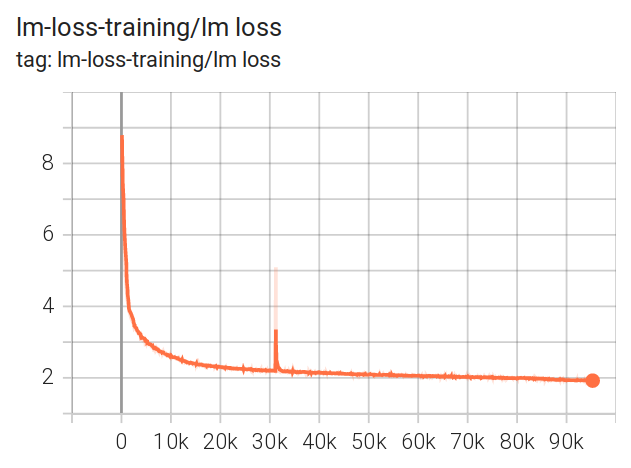
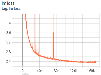
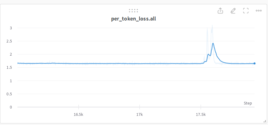
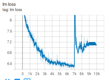
Compare the original run traces
These snapshots come from different model sizes, datasets and logging systems. Compare shapes within each plot, not absolute loss or horizontal units across plots. Unsmooth and smoothed traces can differ; read the surrounding run logs before assigning a cause.
A run can fail without a sharp spike
A plateau can be ordinary diminishing returns, underfitting, a schedule issue or an implementation bug. Sustained upward drift and increasing oscillation require investigation even without a single dramatic event.
Compare a smaller known-good run. Check gradient/update norms, activation/logit scales, precision, source losses, initialization, normalization and parallelism. Reproduce from a common checkpoint before combining interventions.
Bekman's pre-BLOOM account describes several unsuccessful 104B attempts and a later successful 176B recipe with BF16, cleaner data and embedding normalization. This is a combined recipe change, not a controlled proof that one of those changes alone fixes divergence. Original run accounts ↗
A checkpoint contains more than weights
Restore model weights, optimizer moments, scheduler position, scaler, RNG streams, loader cursor, sampler state and mixture counters. Include packing buffers, prefetched work and distributed ownership when they affect the next batch.
Test an uninterrupted branch against an interrupted-and-restored branch early. Compare sample IDs, target-token counts, source ratios, losses and updates. Define whether the backend promises exact replay or statistical equivalence; do not silently demand bitwise identity from nondeterministic kernels.
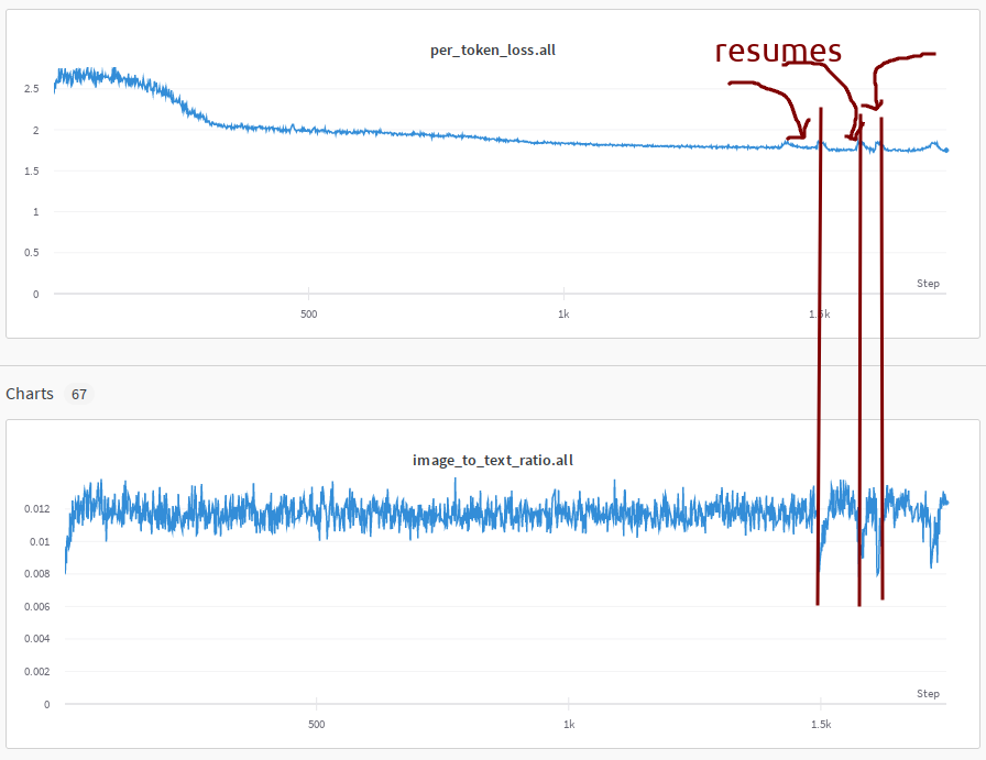
Check log lineage too. A rollback can leave stale future observations in a dashboard. New and old branches must not masquerade as one continuous trajectory. Preserve the parent checkpoint and data exposure rather than relying on a plot's step number alone.
Repeated data can look like progress
If the loader restarts from an old cursor, already-seen material can produce a lower training loss. When fresh data returns, the mean rises. That rise may end a false improvement rather than begin a new instability.
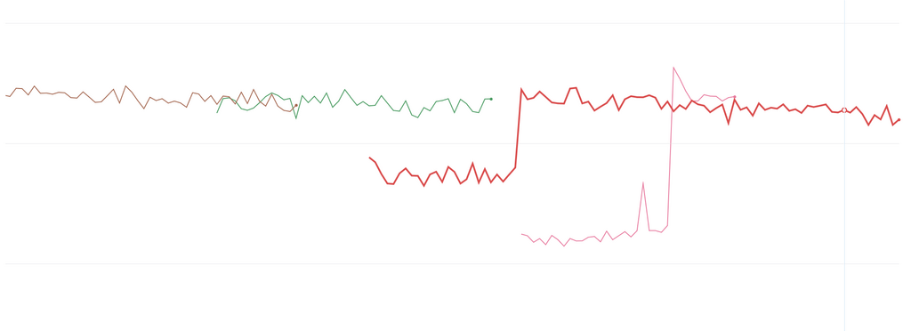
Track document/shard IDs, duplicate exposure and loader position. Keep held-out evaluation independent of the repeated segment. Accidental replay invalidates ablations that assumed equal novel exposure. Deliberate epochs are a different, versioned policy; see source caps and cumulative exposure →.
Separate mixture movement from source degradation
Aggregate loss can move because source losses changed, because composition changed, or both. Log source-specific loss with fixed held-out sets and realized target-token shares. Include web, code, math, multilingual, image-text, synthetic and instruction sources where relevant.
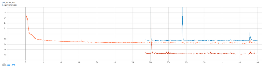
A source-local event suggests inspecting its parsing, labels, length and sampling path. A simultaneous event suggests a shared component, but does not prove one. The same update can affect domains differently.
Change the mixture while domain losses stay fixed
An aggregate can rise without degradation
| Domain | Loss | Target-token share |
|---|---|---|
| Web | 2 | 50% |
| Code | 4 | 50% |
| Aggregate | 3.00 | 100% |
Aggregate=(1−x)×2+x×4=3.00, with code share x=0.50. No domain became better or worse. Increasing code share raises the mean because code has higher assigned loss.
Real comparisons require the same tokenizer, masks, reduction and fixed evaluation sets. Different loss levels do not alone rank domain quality or usefulness.
Make the investigation reproducible
- Mark the event and preserve the preceding checkpoint, batch lineage and full logs.
- Check whether resume, packing, source ratios, precision or throughput changed.
- Compare raw norms, clipping, actual updates, held-out losses and task behavior.
- Inspect a window before the visible event. The last batch need not be its origin.
- Branch a short reproduction with one intervention and a matched control.
- Decide to continue, rollback or change the recipe using recovery and measured cost.
Reducing learning rate or tightening clipping may suppress symptoms while hiding a broken loader or reduction. Keep unsuccessful reproductions. A hypothesis becomes stronger when it predicts a changed outcome, not when it matches one curve's appearance.
Fault tolerance and goodput → accounts for recovery cost. Framework checks → includes state and distributed behavior.
Some failures take a long time to appear
In MoE, track expert utilization, dead experts, padding share, router/logit scale and head gradients. Allocation can degrade before aggregate loss becomes alarming. Identical padding inputs can concentrate on one expert if routing and balancing count them.
The Laguna-related original records expert collapse after hundreds of billions of tokens under mismatched Muon learning-rate and effective-decay scaling. It also records a distinct BF16 LM-head input-gradient all-reduce issue under tensor parallelism as logits drifted upward. FP32 stabilized that reduction.
These are source-specific report observations, not a rule that all MoE failures are Muon problems or all collectives require FP32. Dense early layers can be a recipe choice; they are not a universal cure. MoE owns the detailed allocation, numerical and feedback mechanisms →
Stress a recipe before trusting a smooth pilot run
A short small-scale run may not expose instability that appears after a long production plateau. Qwen raises the learning rate and holds it constant to make failure modes visible at moderate scale. This tests a stability margin; it is not the production schedule.
The main comparison uses a 28-layer 25B-A3B MoE, the same batch and a global gradient clip threshold of 0.5. A loss spike exceeds a 201-step rolling median by more than 0.1. They also track pre-clip p99.9 norms, threshold crossings and maximum activations.
| Setting | 2× optimal LR | 4× optimal LR |
|---|---|---|
| Qwen3.5 structure + AdamW | 4.3 | 183 |
| Same structure + Muon | 0.2 | No clipping-threshold crossing; spike count not specified here |
| Muon + GR | 0.2 | 0 loss spikes; no clipping-threshold crossing |
At 4× LR, AdamW crosses the threshold on 213 of 19,932 steps. The prose describes clipping as continuous, but that count is about 1.07% of steps, not clipping on every step. Keep the numerical evidence rather than repeating the stronger phrase.
To isolate the gate, they hold AdamW, structure and data order fixed and toggle GatedNorm at 3× optimal LR. Spike rate falls from 32.0 to 3.2 per 10,000 steps, and threshold crossings fall from 256 to 20. This isolates the gate more cleanly than comparing full recipes.
The authors propose that multiplicative gates provide the rescaling that ungated networks otherwise obtain through large activation outliers. The experiments support reduced outliers and instability. They do not prove a universal causal theory of every loss spike.
They also compare the first 276B production tokens with shared optimizer, data order and LR schedule. Adding GR improves loss by 0.026; the full recipe improves another 0.032. Relative to Muon alone, gated configurations have approximately 4.3–4.7× lower rolling gradient-norm standard deviation. The final recipe reportedly trains without loss spikes or abnormal gradient norms, without explicit qk-clip or SwiGLU-clip.
Do not translate this into “no clipping of any kind”: the controlled experiments retain a gradient clip threshold, which often never engages. Explicit activation/logit clipping and global gradient-norm clipping are different interventions.
Retest after post-training
Two shortcuts survive early checks but fail later. NoPE in retrieval layers increases endless generation after post-training. Reading only two GR branches preserves early loss and benchmarks but reduces later quality. A useful evaluation ladder therefore includes base loss, downstream tasks, matched pilot post-training, generation termination and the intended serving regime.
For an adaptation, predeclare spike definitions and monitoring windows; save full logs; vary LR under controlled conditions; then confirm the result at production settings. A high-LR failure is not proof that the nominal recipe will fail, and a stress-test success is not a generalization guarantee. GR mechanism → · Optimization-region evidence →.
Qwen3.8-Next architecture report, §3.3, Figures 10–13, pp. 19–22 (26 August 2026) ↗.
Smooth loss does not certify shortcut resistance
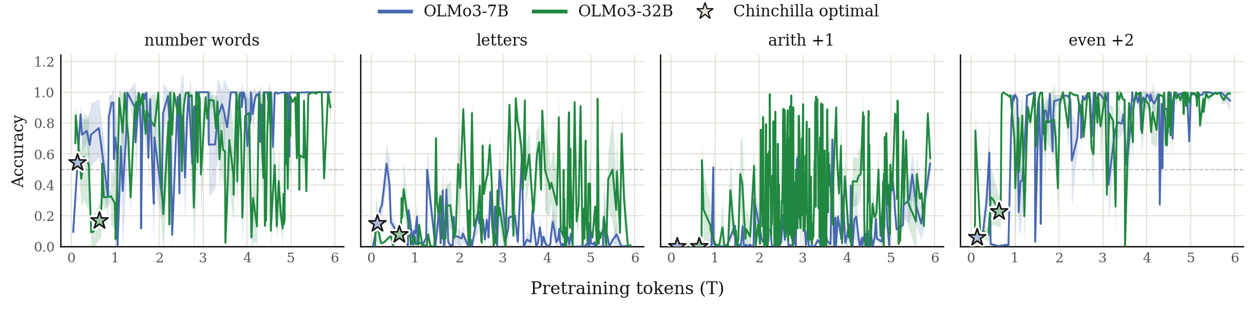
Once run correctness is established, a different problem remains: what computation does the model prefer when a tempting pattern conflicts with the task? Wen et al. study that question across saved pretraining checkpoints.
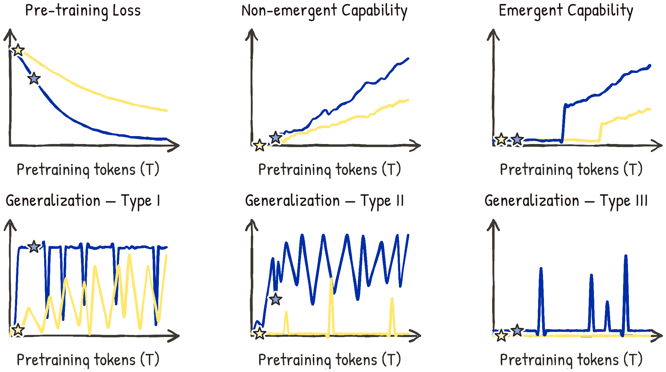

The authors call behavioral switching mode-hopping. That name does not prove two discrete internal states or an identified circuit replacement. Capability, shortcut resistance and adaptability remain separate evaluation targets. Generalization Dynamics of LM Pre-training ↗
Make the shortcut conflict with the task
The study uses general-pretraining OLMo3-7B/32B and Apertus-8B/70B checkpoints. Main dynamics exclude midtraining and long-context stages. The authors report four random seeds. Their main probing families are:
| Probe | Competing shortcut | Task behavior |
|---|---|---|
| Flipped labels | Use a familiar label meaning | Infer the demonstrated mapping |
| Repeated answers | Copy a repeated answer | Solve the new instance |
| Successive answers | Continue an answer sequence | Compute even when the sequence breaks |
| Truth/plausibility | Prefer a believable statement | Recognize surprising truths/misconceptions |
| Cognitive reflection | Give the intuitive wrong answer | Solve the underlying relation |
| Multi-hop persona QA | Use disconnected biographical cues | Infer identity and related facts |
For an arithmetic illustration, demonstrations answer 1, 2, 3; the next problem is 68−60. Continuing the pattern gives 4, while calculation gives 8. Correct ordinary arithmetic examples would not separate those behaviors.
Most tests compare predefined answer-span probabilities rather than grade free generation. Persona QA uses generation with five questions per persona, sampled 200 times each. Demonstrations are resampled across the four evaluation seeds. Span probability needs consistent tokenization/scoring; the pairwise margin is not unrestricted generation accuracy because a third answer can win.
The paper also studies function/city out-of-context reasoning after fine-tuning and broader misalignment after insecure-code tuning. These are separate fine-tuning probes, not extra evidence that an output reveals its internal reasoning process.
Inspect three reported checkpoints
Observe collapse and recovery without interpolation
2.17T · 81% · Before collapse. OLMo3-32B, arithmetic answer-sequence probe. Neighboring observations are 20B training tokens apart, not consecutive optimizer steps.
Only three reported observations are shown. Dashed connectors are visual guides, not intermediate measurements. The 0% point is a result on this shortcut-conflict probe, not evidence that all arithmetic capability disappeared.
| Pretraining tokens | Reported accuracy |
|---|---|
| 2.17T | 81% |
| 2.19T | 0% |
| 2.21T | 81.7% |
What the stability checks do and do not exclude
Common benchmarks remain comparatively stable while these conflict probes fluctuate. Continuous probability margins also fluctuate, so hard accuracy's zero crossing is not the whole explanation.
The single-step experiment restores Adam state, samples OLMo3 data and varies batch size and learning rate. Changes on the suite are small even at the tested learning rate of 10⁻². This establishes local stability for those tests, not that optimization is irrelevant over long intervals.
Averaging five checkpoints mitigates but does not eliminate mode-hopping in the tested recipe. The paper's averaging figure is Figure 11; the nearby prose links Figure 12 inconsistently. Do not generalize the tested outcome to every averaging policy.
Cross-dataset correlations are often low. Larger models show more consistent behavior across datasets in these tests, but can still fluctuate. Equal-FLOP comparisons in Appendix H do not show a generalization advantage for larger models. Capacity is not a cost-free fix.
Compare adaptation from two base checkpoints
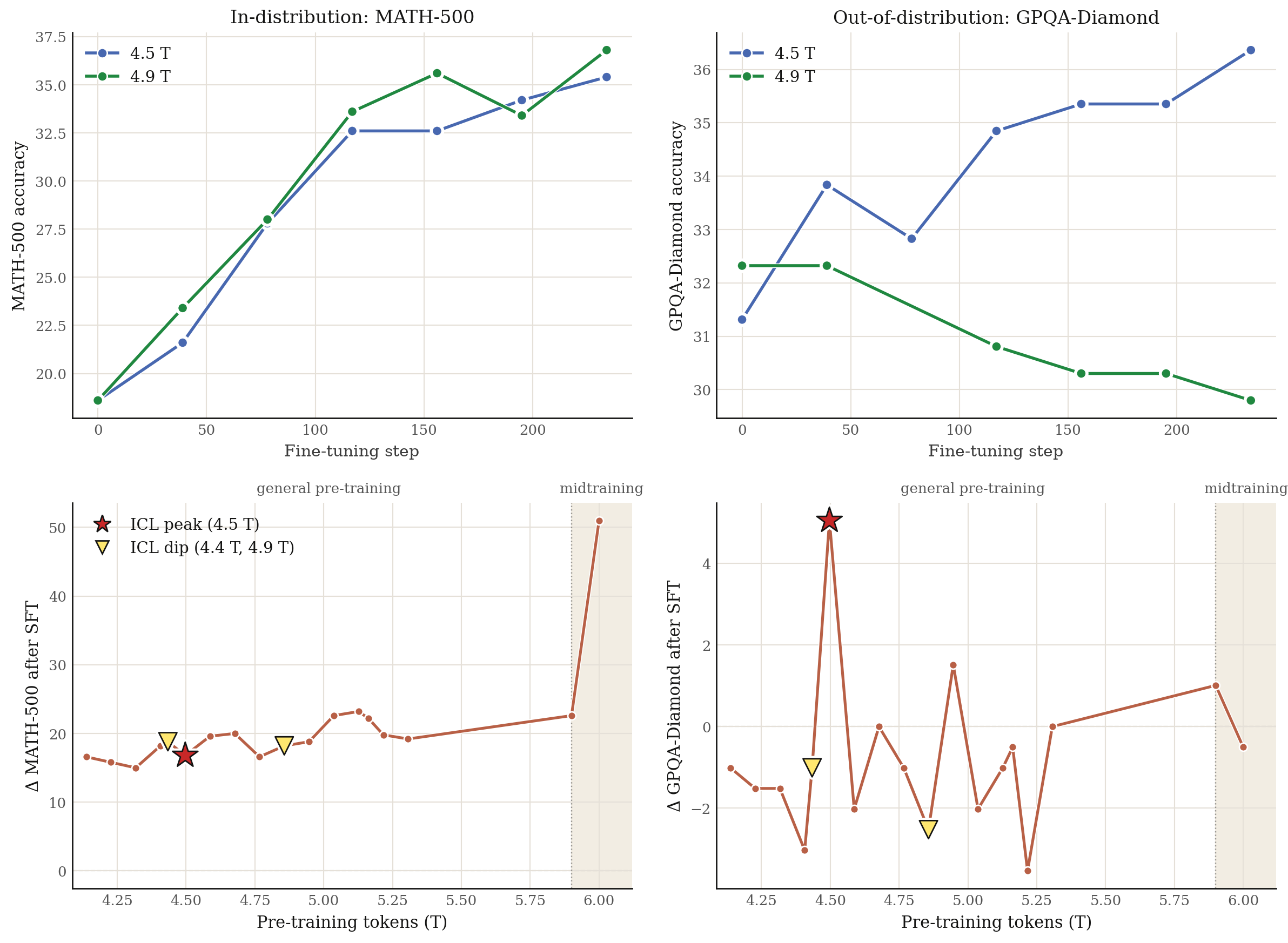
The authors select 4.5T and 4.9T OLMo3-32B bases using their diagnostic suite, then compare post-training. The earlier candidate has stronger suite behavior. The important test is whether this ranking transfers outside the selection probe.
Keep base lineage separate from the adaptation metric
GPQA-Diamond after math SFT
Earlier base: +6.5 percentage points. Science reasoning transfer, not the in-domain math score. Bars use the same 0–100% scale. These are separate experiments, not two terms of a single quality score.
| Metric | 4.5T base | 4.9T base | Difference |
|---|---|---|---|
| GPQA-Diamond after math SFT | 36.3% | 29.8% | 6.5 pp |
| Robustness to prefilling attacks after general SFT | 53% | 21% | 32.0 pp |
General SFT uses 49K non-safety examples from official OLMo3 post-training data and 1K safety examples from STAR-1. A prefilling attack supplies an initial assistant continuation intended to steer behavior. Robustness measures the evaluated attack setup, not all safety.
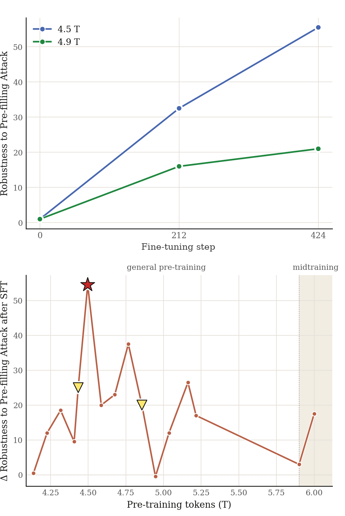
This supports checkpoint selection in the tested OLMo3-32B setting. It does not establish that earlier bases generally win, or that the same ranking survives every SFT/RL budget and data recipe.
Capacity competition remains a hypothesis
The authors propose that shallow pattern computations and generalizable computations compete for limited capacity. Different training-data windows may change which computation dominates output.
Behavioral evidence does not reveal whether a useful circuit was overwritten, became harder to activate or lost a prediction-time competition. The paper does not establish causal circuit replacement. Preserve the distinction between measured switching and this explanation.
Data selection is promising but preliminary
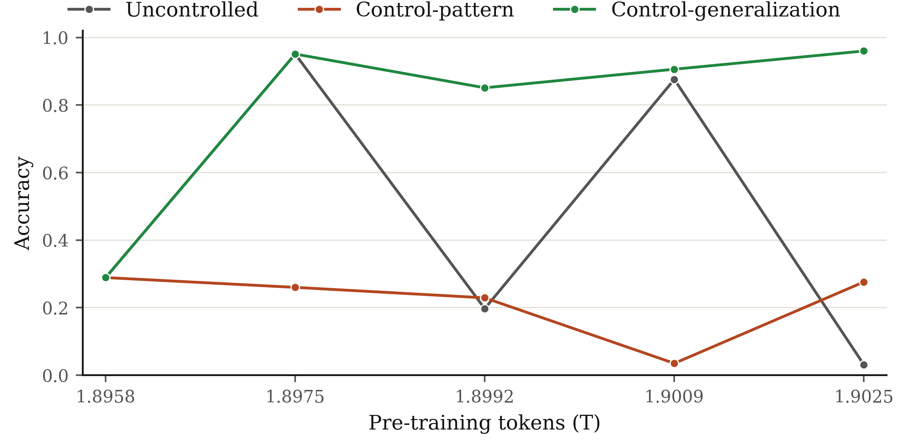
The authors know which windows improved or harmed this probe in the original run. They select continuation subsets retrospectively. The experiment concerns one arithmetic probe and an intermediate OLMo3-32B base.
This is not a classifier that labels arbitrary documents as generalizable. A prospective pipeline needs unrelated held-out probes and trade-off checks. Stabilizing one chosen behavior can harm another. Controlled data-mixture search →
Choose a base through held-out transfer
Use the following as an engineering adaptation, not the authors' exact protocol.
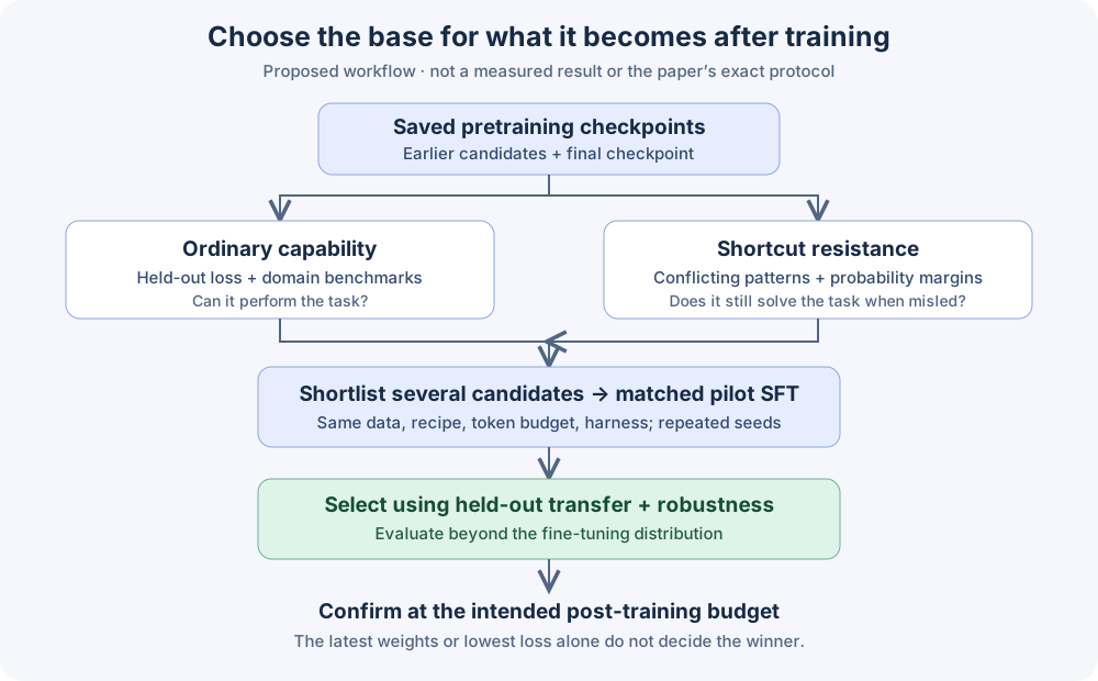
- Save several viable bases with full state and data lineage.
- Track fixed held-out NLL, domain capability, conflict margins and a generative audit.
- Shortlist across domains and prompt variants; avoid a one-probe winner.
- Run matched pilot SFT with identical examples, masks, token budgets, recipes and harnesses. Repeat seeds when feasible.
- Select using held-out transfer and relevant robustness constraints.
- Confirm at the intended post-training budget. Different learning curves can reverse the pilot ranking.
For coding, possible probes include repeated demonstration outputs, misleading templates and short-function adaptation evaluated on held-out repository tasks. These are suggested adaptations, not demonstrated findings from this study.
Do not select a proxy after seeing its winner
Appendix I tests activation/gradient spectrum metrics and gradient similarity. Correlations depend on dataset and layer. Selecting the best layer gives even a random baseline a correlation around 0.4. This selection effect prevents treating the winning layer's correlation as clean prospective evidence.
High and low complexity can both accompany good behavior. A gradient norm, effective rank or sharpness proxy cannot replace held-out task evaluation. Fix proxy choices before the final comparison; account for uncertainty and repeated selection.
The study covers two model families and several templated probes. Selected post-training evidence focuses on OLMo3-32B. Correct answers do not prove a specific reasoning mechanism. Generalization is task-dependent, so keep capability, shortcut resistance, adaptation and run correctness as separate measurements.
References and connected topics
Wen et al., Generalization Dynamics (27 September 2026) ↗ · Paper PDF ↗ · Stas Bekman: training loss patterns ↗ · PyTorch clipping contract ↗
MoE stability → · SFT → · Ablation design → · Inference-aware budgets → · Smol development loop →
Paper images are selected attributed research excerpts for commentary. The arXiv distribution license is not an open reuse license. Original axis/legend limitations remain visible. The parameter and recovery examples are synthetic explanations, not additional experimental evidence.