Scaling Laws
A scaling law answers a resource question—not “how large should every model be?”
On this page
Training compute can buy a larger model, a longer training stream, or a better recipe. These choices compete. A scaling law estimates their trade-off from controlled smaller runs. It is useful only when its variables, objective and extrapolation range match the proposed run.
Start with pretraining allocation. Then account for finite novelty and deployment cost. The later decomposition and coupled-surface sections explain why one fitted power law can hide several bottlenecks.
Start with the objective
Training-compute optimality means the lowest validation loss for a fixed training FLOP budget. Deployment optimality may accept more training to reduce recurring inference cost. A downstream reasoning score, a weighted domain NLL suite and general text NLL are also different objectives.
Do not call a run inefficient without saying which cost and outcome you are comparing. A small, heavily trained model can be off the pretraining frontier and still be the better product choice.
Name the quantities before fitting
| Symbol | Meaning | Important distinction |
|---|---|---|
| N | Model parameters | Total versus non-embedding; active versus stored for MoE |
| D | Processed training tokens in the allocation law | Not necessarily unique tokens |
| U_D | Unique useful tokens | Deduplication and source quality affect novelty |
| C | Training FLOPs | Not elapsed time or dollars |
| B, T, K | Batch samples, optimizer steps, processed samples K=BT | Convert sequences to tokens explicitly |
| E | Fitted constant loss floor | Not measured entropy of an ideal distribution |
Attention length, embeddings, recomputation and other operations change this accounting. Optimizer and communication overhead change elapsed time. For MoE, active parameters approximate arithmetic, while total parameters affect memory and stored capacity. See Distributed Training → and MoE →.
Read a power law above its floor
A multiplicative scale increase gives a predictable fractional reduction in the reducible term. Absolute improvement diminishes. Very small runs can be noisy or unstable; very large runs can hit data or objective saturation. Fit the regime supported by observations, not all points automatically.
Two explanations are useful hypotheses. A structured data manifold can permit progressively finer approximation with capacity. A heavy-tailed distribution of skills can make common patterns arrive early and rare patterns arrive late. Neither is a settled universal mechanism. The quantization model makes the second idea explicit.
For a pure reducible power , rescaling x by λ>0 multiplies f by . Power laws have long tails, scale invariance and simple resource algebra. They are useful first models, not a guarantee against characteristic scales or exponential saturation.
2020: capacity and sample efficiency
Kaplan et al. observed smooth loss scaling with model size, data and compute. Larger models were more sample-efficient. Their compute-allocation summary puts more growth into capacity: , .
A tenfold compute increase therefore gives about 5.4× parameters and 1.9× tokens under that fitted regime. This encouraged large models trained on relatively short streams. It is a result of a recipe and fitting method, not a constant of nature. Kaplan et al. ↗
2022: balance capacity and tokens
Chinchilla used fixed-size training curves, equal-compute sweeps and a joint parametric fit. Its empirical conclusion was much closer to equal growth in parameters and tokens. Many preceding large models had too few tokens for their training compute.
The familiar D≈20N rule gives 20B tokens for 1B parameters, 140B for 7B, and 1.4T for 70B. It is an approximate reference from that study. Different fits need not preserve a constant ratio. Hoffmann et al. ↗
Derive the fixed-compute optimum
Differentiate with respect to N. At an interior optimum, . The weighted reducible terms balance, not necessarily the raw terms or token/parameter counts.
When , both exponents approach one half. If , varies as . Memory limits, discrete architectures and a finite corpus can move the feasible optimum to a boundary.
Small allocation implementation
def allocate(C, A, B, alpha, beta):
    N = (alpha*A/(beta*B))**(1/(alpha+beta))
    N *= (C/6)**(beta/(alpha+beta))
    return N, C/(6*N)
Positive inputs only; units must match the fitted amplitudes. This does not estimate A, B or the exponents.
Move along an equal-compute curve
More capacity means fewer tokens
Move the chosen allocation; inspect loss at a fixed normalized budget.
N=10.000, D=10.000, 6ND=600. Loss=1.7962; best on this curve=1.7962 at N=D=10. Blue: chosen point; gold ring: optimum.
Assigned , , . Both axes are logarithmic. Units are normalized, not billions of real parameters or tokens. The outer exponent changes loss, not this fixed-inner-parameter optimum.
Why fitted frontiers disagree
Kaplan and Chinchilla used different scale ranges, training schedules, extrapolation procedures and parameter conventions. Embeddings are a large share of small models. Counting total versus non-embedding parameters changes a proxy fit; it is not a full explanation of all disagreement.
A small slope error becomes large across several orders of magnitude. Later reconciliation and replication studies are useful checks on methodology. Compare several fitting views, consistent parameter counts and a larger held-out run before choosing a final allocation.
Convert compute into a first budget
| Question | Calculation | Result |
|---|---|---|
| 7B parameters, 1T tokens | FLOPs | |
| FLOPs, 10B parameters | 1.67T tokens | |
| FLOPs under | 28.9B parameters; 577B tokens | |
| 64 GPUs, 30 days, 989 TFLOP/s peak, utilization 0.35 | FLOPs; about 21.9B parameters and 438B tokens under the rule |
The final row multiplies GPU count, elapsed seconds, per-GPU peak FLOP/s and utilization. Use realized training throughput and recovery overhead. A peak spec times an assumed utilization is only a scenario. The original note used FLOPs. Direct multiplication gives FLOPs, rounded to three significant figures in this table. Both allocations round to about 21.9B parameters and 438B tokens. Long context and sparse hardware behavior require a more detailed accounting model.
Count novelty separately from exposure
A 2T-token unique corpus seen three times has R_D=2 and D=6T. It does not contain 6T unique tokens. For small repeats the effective-data law initially behaves like extra data. At large repeats it approaches .
Muennighoff et al. also discount excess model capacity relative to the compute-optimal model for the unique corpus: . Their fitted law uses effective N′ and D′ rather than raw counts. The model-size discount applies in its defined excess-capacity regime; a negative excess ratio is not a repetition amount. Data-constrained language models ↗
Watch repeated tokens lose marginal value
An extra pass is not an extra corpus
Both bars use the same fixed linear scale.
U=1, r_D=4, R=2. Marginal effective tokens per extra pass: =0.607. No repetition gives D′=1. The ceiling is 1+4=5, not unlimited growth.
This is the assigned exponential-discount model, not a measured corpus or an overfitting curve. It can saturate; it cannot by itself make validation loss rise.
Model memorization without extrapolating forever
The final term grows with repetition and capacity relative to unique data. It can represent a local validation-loss turn upward, unlike effective-data saturation alone. P, δ and κ must be fitted. It is not an established identity or a law that every large model must overfit faster.
A positive unbounded power penalty predicts divergent loss for unlimited repetitions. Do not extrapolate that limit as fact. Compare saturation and overfitting forms on held-out repeated-data runs. Regularization can change the fitted behavior, but stronger decay can also underfit or damage rare knowledge.
Make repetition source-specific
Track source-level passes, exact and near duplicates, semantic redundancy, validation loss by domain and target coverage. Mathematical proofs, boilerplate, code templates and benchmark-like items have different novelty and contamination risks. Their useful epoch limits must be measured, not inferred from the labels alone.
Data-constrained means constrained by quality, diversity, rights, deduplication and coverage—not only bytes. “Clean data shifts the curve” is a hypothesis to test under a fixed evaluation. A global token count can conceal a few heavily repeated sources.
Nanbeige’s original report describes a 12.5T filtered pool, a 6.5T higher-quality subset repeated for at least two passes, and a 23T final stream. It deliberately changes the mixture during FG-WSD. That is a joint data/schedule intervention, not evidence that repeating any 6.5T corpus will have the same effect. Complete pipeline →
Tune weight decay together with repetition and model size rather than treating its effect as independent. Compare data quality at fixed N, raw D and evaluation. A higher D/N can reflect useful diverse exposure or low-novelty repetition; the ratio alone cannot distinguish them. Data mixture objectives → · Duplicate and memorization controls →
Change the objective, not the meaning of optimal
Training is paid once; inference recurs. A smaller model trained longer can reach a useful quality target at lower lifecycle cost. Extra tokens beyond the pretraining frontier may still help; they are less efficient than changing capacity under that particular training-only budget.
The rough phrase “training cost ≈ inference cost” is not an optimality theorem. The optimum depends on marginal costs, demand, latency, hardware and the loss surface. Overtraining describes a reference comparison, not a promise of improved quality or a diagnosis of harmful overfitting.
| Constraint | What to measure | Why parameter count is insufficient |
|---|---|---|
| Latency | Prefill and decode latency at the intended batch/context | Serial depth and kernel utilization change runtime |
| Memory / local deployment | Weights, KV cache and peak working memory | MoE active count omits stored experts |
| Recurring demand | Expected served work over the deployment lifetime | Training is paid once; serving repeats |
| Adaptation | Fine-tuning quality and cost at matched data | Heavy pretraining is not a universal adaptation gain |
These are constraints to test, not guaranteed benefits of more tokens. Serving economics → · Small and on-device recipes →
Read heavy-training examples with their denominators
| Model / regime | Reported tokens and denominator | Interpretation |
|---|---|---|
| Llama 3 8B | TPP | Far beyond the rough 20 TPP reference; original report discussion quotes ≈200B compute-optimal tokens |
| DeepSeek-V3 | active TPP | Active TPP is not a fitted dense-model optimum |
| GLM-4.5 | active TPP | Stored capacity and serving behavior differ |
| MAI | 100–200 TPP ablations; 500–1,000 production | Training density can change architecture rankings |
| Nanbeige4-3B | TPP | A small dense model with exceptional training investment |
| Qwen3 | 36T across a staged family | Do not assign one family-wide TPP without a size/stage denominator |
The Llama 3 discussion reports continuing improvement at very high token density and motivates smaller models through inference efficiency. This is not indefinite linear improvement or proof that every benchmark tracks NLL. Nanbeige’s targeted reasoning strengths also do not mean a 3B model universally beats larger models.
The Smol Training Playbook treats scaling laws as planning priors for useful small models. Epoch AI’s 2025 trend analysis reports rising tokens per active parameter and roughly 20× the Chinchilla reference in recent open models—about 400 TPP if the comparison starts at 20. These historical observations are not today’s measured ecosystem-wide ratio.
Meta Llama 3 announcement ↗ · DeepSeek-V3 report ↗ · GLM-4.5 report ↗ · Qwen3 report ↗ · Epoch AI: August 2025 trend ↗
TPP means tokens per parameter. Dense TPP is ; active TPP is . GLM’s 23T is a multi-stage budget. Family/stage totals are not necessarily the same exposure for every released checkpoint.
Include the rest of the train–infer–think pipeline
A pretraining fit does not price continued pretraining, context extension, SFT, RL or reasoning tokens. High TPP can mean useful diversity or repeated low-novelty content. It does not reveal which. Long-context serving also includes cache and attention costs, not only active parameter FLOPs.
Overtraining may change adaptability; post-training behavior needs separate measurements. Choose a base model for the complete pipeline. A reasoning-time compute objective is different from minimizing pretraining NLL under 6ND. Keep those studies separate before combining their costs.
The named studies ask different questions. Sardana et al. add deployment demand to model/data allocation. Gadre et al. study overtrained loss and downstream-task prediction. Train-to-Test scaling jointly budgets model size, training tokens and repeated inference samples. Each empirical scope is distinct; none proves that a high TPP always improves adaptation.
Beyond Chinchilla-Optimal ↗ · Gadre et al.: overtraining and downstream tasks ↗ · Test-Time Scaling Makes Overtraining Compute-Optimal ↗ · Reasoning and test-time budgets →
Decompose the loss before proposing a law
Su Jianlin inserts idealized training optima between achieved training loss and target-distribution loss. Let L_target be achieved target loss; L_train achieved training loss; L_best the architecture’s best training loss; and L_∞ the unrestricted training floor.
The identity is exact if these quantities are defined consistently. Its power-law parameterizations are hypotheses. Under nested feasible classes and true global optima, the architecture and optimization gaps are nonnegative. The target-minus-training difference need not be: a target distribution can be easier than the training set. The original general nonnegative-gap claim needed this correction.
The training floor depends on the training distribution and class convention. It is not automatically the irreducible entropy of the inaccessible ideal distribution. These gaps interact: architecture affects optimization and generalization. They are not independently measurable causes simply because they sum to loss. Deconstructing scaling laws ↗
Build the accounting identity
Add differences between nested losses
Use the signed alternative to see why the identity does not imply positive generalization.
No components added yet.
Assigned training loss 2.2, best architecture loss 1.8, unrestricted training floor 1.4; target loss 2.5. The target distribution is harder: the data difference is +0.3. These optima are conceptual in real neural training; the bars are not measured independent causes.
One algebraic pattern connects the trade-offs
At the optimum, . The increasing and decreasing contributions balance after weighting by slopes. Power-law inputs can therefore produce power-law optimal allocations. This mathematical closure explains recurring formulas; it does not establish that the proposed input terms describe training.
Balance travel and update precision
More steps or a larger rate reduce the first term; an overly large rate increases the third. After optimizing η, combine the travel and update terms.
A longer horizon changes the derived frontier.
Longer runs permit a smaller optimal rate under this model. A fully tuned frontier need not retain η as an independent fit variable. This is not a guarantee that a real optimizer has these terms or remains stable at the derived rate. Optimization and joint batch/LR experiments →
K means processed samples, not unique data
If and , then , , , and the optimized gap scales as . The last rate result uses ; it does not hold at fixed B automatically.
For 1,000,000 processed sequences, B=100 gives T=10,000; B=1,000 gives T=1,000. K is unchanged. If each sequence has S fixed tokens, total processed tokens are SK. With variable lengths, sum actual valid tokens. Repeated examples count again in K, but not in unique data.
Agreement with empirical exponents is suggestive, not confirmation of the mechanism. Tune on controlled proxy runs and test a near-optimal region instead of using this as an uncalibrated batch recommendation.
Model size also changes the optimization terms
The preceding batch derivation holds architecture fixed. The loss-decomposition blog then lets N change the three coefficients, while holding the exponents fixed. This is a hypothesis, not proof that larger models necessarily introduce more gradient noise.
The first rate optimum holds T and B fixed. The later expressions jointly optimize rate and batch at fixed K. At that joint optimum, each reduction balances its opposing cost. Requiring both optimal batch and optimal gap to be independent of N gives the following conditional simplification.
The rate can still depend on size when batch and optimized gap do not. Assigning gives the ratios below. These are normalized illustrations, not measured tuning results.
| Change | Rate ratio | Batch ratio | Optimization-gap ratio |
|---|---|---|---|
| Processed samples K ×16 | 0.5 | 4 | 0.5 |
| Parameters N ×16 | 0.5 | 1 | 1 |
Integer batches, memory limits, stable-rate ranges and schedules can move the optimum to a boundary. Calibrate the hypothesis on controlled runs before using it.
Allocate width and depth under a parameter budget
With both exponents one, width and depth scale as , and the gap as . This derives a shape rule from assumptions, not a proof of universally optimal transformer shapes. Kernels, depth stability, attention/FFN ratios and memory change the feasible architecture.
Balance optimized training and architecture
Using and gives , and . The near-equal allocation resembles Chinchilla. It does not prove that Chinchilla’s fitted data term is this optimization gap.
The same conditional model also predicts how tuning changes along this compute frontier. Substitute the optimized size and exposure into the preceding rate and batch laws.
With the assigned size exponent 0.25, a 128× compute increase gives the following ratios. Each row changes jointly; these are not independent hyperparameter sweeps.
| Quantity | Ratio at compute ×128 |
|---|---|
| Parameters N | 8 |
| Processed samples K | 16 |
| Batch B | 4 |
| Optimizer steps T | 4 |
| Learning rate η | ≈0.2973 |
| Combined optimization + architecture gap | 0.5 |
The compute factor must stay constant across runs. Sequence length, attention cost, sparse routing, utilization and wall-clock overhead can invalidate that condition. A fitted learning-rate exponent also depends on the optimizer and schedule. This calculation is not a universal scaling recipe.
Stored capacity does not replace active computation
Without the active-capacity penalty, a simplistic product law can make pathological trade-offs between stored capacity and active computation. At fixed N_act, increasing sparsity adds stored capacity, but it also changes routing, communication, imbalance, utilization and memory.
This equivalent count rewrites the product term as a dense-shaped power law. It is not a measured equivalence between two architectures. If , the expression reduces to . Assigned active/total counts of 4/36 give . The same product term can therefore occur at different active costs. The extra active-capacity penalty breaks that equivalence for the full gap. Routing and hardware costs remain separate.
PKM, UltraMem, Over-Encoding and Engram can be viewed as sparse retrieval capacity: select a few stored vectors instead of computing every weight. This analogy is not architectural identity. Under fixed active compute and memory, experts and retrieval can have an interior allocation if their distinct marginal improvements justify it. The exact additive model remains a hypothesis. Routing, balancing and expert parallelism →
Divide storage between experts and memory
The preceding sparse-capacity model leaves an allocation question open. At fixed active work and total storage, should extra parameters be inactive experts or retrieved vectors? Su Jianlin proposes separate power-law terms for these two sources of capacity. This is a modeling hypothesis, not evidence that any fixed mixture wins.
First count each component once. A counts dense parameters plus active experts; X counts inactive experts; M counts stored memory vectors. These are parameter counts, not bytes. In this model, A excludes retrieved vectors because they do not perform an expert matrix multiplication. Retrieval, selection and fusion still require real computation.
Fixing A makes the active-capacity penalty constant. The proposed architecture gap then reduces to two decreasing terms. Moving storage toward one term reduces the other term's capacity.
The fixed-sum constraint differs from the earlier fixed-compute product constraint. Differentiation balances the marginal improvements, not the two losses themselves.
Physical counts add a restriction: . Neither side can contain fewer than the active base. The unconstrained root can fall outside this interval. In that case the feasible optimum is an endpoint: all additional storage goes to one component. An interior mixture is therefore possible, not guaranteed.
For equal exponents , the unconstrained root has a closed form: . For unequal exponents, solve the monotone equation numerically. Real expert counts are discrete; evaluate feasible neighbors around a continuous prediction.
| Extra storage | N_moe | N_mem | |
|---|---|---|---|
| All memory: X=0, M=16 | 8 | 24 | 3.5000 |
| Mixture: X=12, M=4 | 20 | 12 | 2.0000 |
| All inactive experts: X=16, M=0 | 24 | 8 | 2.1667 |
Here gives within the feasible interval . The mixture is best under these assigned coefficients. Changing the coefficients can move the optimum to a boundary. Fit these terms with controlled architecture experiments before using the prediction. Equal parameter counts also need not mean equal memory bytes or runtime. Source: memory-layer hypothesis ↗
A local repetition penalty gives a fragile epoch rule
This particular model predicts more optimal epochs for a smaller corpus. Other empirical work gives the opposite trend. Its unbounded repetition penalty is also implausible as a universal limit. Constraints such as requiring at least one full pass can clip its optimum. Keep it as a local testable hypothesis, not an epoch policy.
The blog relaxes the penalty's dependence on corpus size instead of tying it to the epoch count alone. Here s controls the optimization decay, t the repetition growth, and r the corpus-size dependence. The original penalty is the special case . The sign of the epoch trend now depends on r, not merely on whether repetition has a cost.
| Corpus dependence | Epoch trend | Assigned example: U grows from 1 to 16 |
|---|---|---|
| Optimal epochs decrease | r=1: K grows 1→4; epochs 1→0.25 | |
| Optimal epochs stay constant | r=2: K grows 1→16; epochs 1→1 | |
| Optimal epochs increase | r=3: K grows 1→64; epochs 1→4 |
The examples assign a=b=1 and , so . These are unconstrained mathematical examples, not recommended training budgets. The first row falls below one full pass at U=16; a full-pass requirement moves that optimum to K=U. The generalized penalty still diverges with unlimited exposure. It explains how assumptions can reverse the prediction; it does not validate any trend. Source: optimal-epoch hypothesis ↗
Test slope changes instead of assuming them
The decomposition blog suggests coefficients represent engineering efficiency and exponents represent problem difficulty. Different exponents imply an unbounded relative reducible-loss advantage asymptotically. That is an argument for testing shared slopes, not proof that architecture or optimization cannot change exponents.
Scale range, task distribution and dominant bottleneck can change fitted slopes. Fit shared- and separate-slope alternatives, assess uncertainty and validate at larger held-out scales. Avoid a large combined formula with many correlated terms before nested experiments support its parts.
2026: ask whether model and data interact
The additive law forces marginal capacity value to be independent of data. Videau et al. find systematic boundary residuals and predominantly negative mixed derivatives on their main grids. They estimate derivatives using moving least squares and a differentiable Gaussian-process surrogate; small first-order cross-slopes can conceal second-order interaction.
For 0<k<1 the mixed derivative is negative: more data makes extra capacity more valuable, and vice versa. k=1 is additive; k>1 gives the opposite cross-effect. Both first derivatives remain negative for any k>0.
A negative additive interaction can instead break monotonicity. The outer power avoids that problem. Kaplan had an outer coupling with tied inner exponents; Skaling unties them. Related forms also appear in distillation scaling. The contribution is not the discovery that no one had ever used an outer power. Skaling ↗
Convert log-coordinate derivatives correctly
The numerical estimators fit a surface in log coordinates. A derivative of log loss is not a derivative of loss. Apply the chain rule before interpreting its sign.
Assigned local example: at N=D=L=1, take log slopes −0.2 and −0.3, and log mixed derivative −0.02. The actual mixed derivative is positive:
| Contribution | Value |
|---|---|
| Log mixed derivative | −0.02 |
| Product of log slopes | +0.06 |
| Mixed derivative of loss | +0.04 |
A negative log mixed derivative alone therefore does not establish negative model–data interaction in loss. MLS neighbourhood choices and GP kernel/noise choices also affect the estimated surface. Compare estimators and test the actual converted derivatives.
Compare marginal gains on the same surface
Does data change the value of capacity?
Keep all inner parameters fixed; vary only the outer mapping.
| D | Loss at N=10 | Loss at N=20 | Gain |
|---|---|---|---|
| 1 | 2.3981 | 2.3017 | 0.0964 |
| 4 | 1.9725 | 1.8761 | 0.0964 |
| 16 | 1.7280 | 1.6316 | 0.0964 |
| 64 | 1.5876 | 1.4912 | 0.0964 |
| 256 | 1.5069 | 1.4105 | 0.0964 |
Selected D=16; k=1: doubling capacity lowers loss by 0.0964. Mixed derivative at (10,16)=0.000e+0.
The gain is the same at every D: the additive law forces zero mixed derivative. Inner parameters are held fixed. Different absolute losses between k values are not fitted evidence of which law is better.
The outer exponent does not directly move the optimum
For k>0, is increasing. Under the same constraint, minimizing the coupled loss is equivalent to minimizing its inner sum. The allocation formulas above therefore still apply when A, B, α and β are held fixed.
Fitting a different surface changes those inner parameters, which can move the predicted optimum. On Farseer, derivative estimates give or ; Skaling predicts about −0.11 and additive Chinchilla about +0.03. On SK-Grid, instead predicts an increasing ratio. There is no universal replacement TPP number or universal decreasing trend.
In PDF Figure 6, the GP and MLS curves locate minima on smooth surrogate surfaces fitted to the measured runs. They are not directly measured optimal training runs at every compute budget. The right panel extends power-law fits outside the shaded data range; agreement there is extrapolation, not frontier validation.
Use an L-shaped grid, then test its missing corner
Large-long runs dominate dense-grid compute. Sweep D at small N and N at short horizons; use the coupled form to predict the rest. Reported fitting compute falls from 5.0×10²² to 5.1×10²¹ FLOPs on Farseer and from 3.1×10²¹ to 6.5×10²⁰ on SK-Grid: approximately 10× and 5× respectively.
Both bands still need enough range to identify decay rates. Sparse fitting does not remove expensive validation. Withhold several larger-N, larger-D and far-corner runs deliberately before a frontier commitment.
Keep the Skaling comparisons and their scope
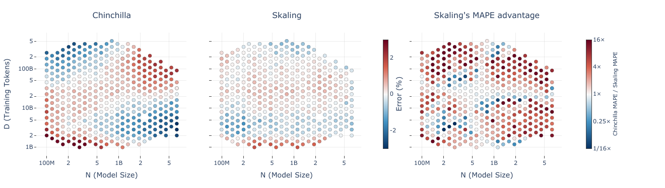
MAPE measures prediction error relative to each measured validation loss. It does not measure the loss improvement from training a model. Measured losses 2 and 4, with predictions 2.2 and 3.6, give 10% MAPE.
Table 1 reports means and standard deviations across five cross-validation folds. The deviations below are not confidence intervals. The far-extrapolation sets contain only seven Farseer runs and three SK-Grid runs. Small far-corner samples limit how broadly these gains can be interpreted. The grids use a prescribed hyperparameter policy, not a new exhaustive tuning sweep at every point.
The study records Farseer’s 404 configurations, mainly 100M–6.4B parameters and 1B–512B tokens, with larger-model checks to 25B; SK-Grid’s 134M–4.9B appendix models and checks to 10.8B; 117 code-domain runs; and 245 replicated Chinchilla configurations. These are not present-day frontier-sized measurements.
| Regime | Farseer | SK-Grid |
|---|---|---|
| Interpolation | 0.77 ±0.04 → 0.41 ±0.05 | 0.81 ±0.14 → 0.33 ±0.11 |
| Larger N | 1.48 ±0.03 → 0.47 ±0.03 | 0.83 ±0.11 → 0.39 ±0.05 |
| Larger D | 1.98 ±0.08 → 0.88 ±0.06 | 1.44 ±0.03 → 0.58 ±0.07 |
| Far extrapolation | 2.46 ±0.19 → 2.31 ±0.18 | 5.17 ±0.28 → 0.70 ±0.39 |
The figure comparison favors Skaling on 76% of configurations, with median 2.2× error advantage. The boundary gains matter more than interpolation fit. On SK-Grid far extrapolation, full/L-shaped Chinchilla give 5.17%/14.63%; full/L-shaped Skaling give 0.70%/1.15%.
A fixed-ratio test uses 14 Farseer D/N rays and eight high-compute held-out points per ray, 112 total. MAPE: Chinchilla 2.34%, Farseer law 0.80%, independent per-ray power fits 0.99%, Skaling 0.60%. Independent per-ray fits are slightly better on the near-optimal-ratio subset, where each recipe receives its own fit. They cannot answer joint allocation questions.
Code and replication sets have weaker coupling: versus roughly in the main grids. Hyperparameter policies can change the observed surface. Extrapolation to 2×10²⁵ FLOPs is far beyond measured budgets around 10²². Version-one SK-Grid run accounting also differs between section 4.1 (134/15 sizes) and appendix E (125/14). Retain that inconsistency rather than choosing an unverified count.
Keep the measured surface tied to its recipe
Appendix E specifies the SK-Grid policy used to generate the measured surface. Its StepLaw coefficients were refitted for this setup.
The reported peak rate increases with token budget. This is a recipe-specific prescription, not the fixed-K optimum derived above. Changing units changes the numerical coefficients.
| Control | Setting |
|---|---|
| Tokenizer / context | Llama 3; vocabulary 128,256; 2,048 tokens |
| Width / depth range | 672–3,264 dimensions; 7–34 layers |
| Data / validation target | 60% DCLM-Edu web, 30% code, 10% math; held-out split of this mixture |
| Optimizer | AdamW; moments (0.9, 0.95); weight decay 0.1; gradient clipping 0.1 |
| Schedule | Cosine; 10% warmup; final learning rate 0.000001 |
Compute caps give larger models fewer token horizons: the smallest row has 16 budgets, the largest only one. This staircase is not a full Cartesian grid. Keep the separate version-one run-count discrepancy visible rather than resolving it by assumption.
The fitted floor is not measured entropy
In the original Farseer fit, Skaling shifts E from about 0.45 to 0.03. This does not demonstrate near-zero irreducible loss. k and E can compensate over an unsaturated range; the observations constrain their sum better than their individual interpretation.
Subtract losses for dominated pairs—where one run has more parameters, more data and lower loss—to remove E from the fitting objective. Appendix F reports Farseer far-extrapolation MAPE of 2.46%→0.79% for Chinchilla and about 2.32%→1.55% for Skaling using this alternative. Some apparent boundary failure is therefore tied to floor identification, not only zero coupling.
Table 9 uses a separate fitting run, so its 2.32% baseline can differ from Table 1’s 2.31%. The paper states this explicitly; the difference is not merely reported precision. On SK-Grid the coupled advantage remains larger. Compare fitting objectives before claiming that one mechanism fully explains another law’s failure.
Fit the shape from ordered differences, then recover the constant from residuals. In Appendix F, X denotes per-token compute F, not total training compute C.
Pair selection also reweights the observations. Dominated-pair fitting is therefore not simply the same objective with one nuisance parameter removed. It can worsen extrapolation: Farseer L-shape Skaling far-error rises from 1.57% to 5.87% in Table 9.
Design a fit that can fail honestly
Keep tokenizer, data mixture, optimizer policy, schedule, context, precision and parameter convention controlled or explicitly modeled. Preserve loss precision. Inspect rising/flattened curves and failed runs instead of discarding them without explaining the selection.
The Skaling fit uses Huber error in log loss with transition , log-amplitudes, analytic gradients with bounded L-BFGS-B, basin hopping with Sobol initialization and 2,000 restarts, with CMA-ES as a cross-check. Its bounds are , , . They are fit constraints, not physical constants.
Compare additive and coupled models under the same objective/optimizer. Report folds, parameter variation, signed residual maps, interpolation, single-axis and far-corner errors separately. Test intended D/N rays and floor-free alternatives. More parameters do not guarantee a stronger baseline: the nine-parameter Farseer form is also harder to fit.
Use nested experiments: tune optimization at fixed data/architecture; study architecture near a tuned regime; study data under controlled optimization; combine only supported terms. Validation NLL is smoother than many generation scores, but the final target still needs downstream checks and uncertainty. A high in-sample R² is not an extrapolation certificate.
| Question | Variables | Transfer check |
|---|---|---|
| Model/data allocation | N,D and processed budget | Validate a larger held-out run |
| Hyperparameter scaling | Learning rate,batch,warmup,decay | Retune or calibrate their horizon dependence |
| Parametrization transfer | Width and weight/update scaling | Check that a proxy optimizer setting transfers |
A correctly sized model can still be poorly optimized. Fit the smallest supported gap model first, derive its constrained optimum, then test new runs near that prediction. Reject terms that imply impossible limits.
Compare curves, not one proxy winner
MAI compares architecture/data candidates on scaling ladders at a matched training density. means the fitted baseline needs 30% more cost to match the candidate. and separate modeling efficiency from actual implementation speed. Recovery and goodput affect the latter.
The original internal NLL target is 0.5 Coding +0.175 STEM +0.175 Math +0.1 General +0.05 Multilingual. It encodes priorities; it is not neutral general quality. A STEM-heavy mixture winning at small scale but losing to a code-heavier one at larger scale illustrates why rankings must be revalidated.
Keep ablation and production TPP distinct. A proxy design win need not survive heavier training, a different mixture or a different kernel implementation. The full report also discusses deduplication, epoch caps and deterministic recovery; those belong with data/run design rather than being reduced to one scaling coefficient.
Refit hyperparameters after changing the architecture and optimizer
Changing the optimizer changes the useful learning-rate/batch region. Changing attention and residual gates also changes the stability margin. Qwen therefore refits its previous hyperparameter scaling law rather than carrying over the old settings. The report does not publish enough fitted coefficients to reconstruct that new law.
They test extrapolation on two deliberately different regimes. A small model with long exposure tests whether a large batch wastes data. A larger model with shorter exposure tests whether the predicted learning rate remains stable. These tests complement each other; neither is a universal proof of transfer.
| Recipe | Global batch, million tokens | Peak LR | Final-window loss |
|---|---|---|---|
| Previous recipe | 12.6 | 3.49e-3 | 1.5774 |
| New predicted region | 25.2 | 5.39e-3 | 1.5702 |
| 1.5× larger batch | 37.7 | 6.92e-3 | 1.5707 |
Each batch uses its paired learning rate from the fit. The comparison tests joint recipes, not batch size with LR held fixed. The 25.2M and 37.7M settings form a relatively flat region. The smaller old recipe is worse by about 0.0072 loss. Report loss and elapsed time separately; equal token budgets do not imply equal optimizer or communication overhead.
A batch ramp starts at 6.3M and increases by 6.3M, reaching 25.2M at 524B tokens. Neither keeping the peak LR nor lowering it for the early batches improves final quality. The ramps end roughly 0.00025 and 0.00035 worse and require 18.8% more optimizer steps. This supports removing batch-size warmup in this recipe. It does not remove learning-rate warmup, which remains visible in their runs.
| Setting | Batch, million tokens | LR | Mean accuracy |
|---|---|---|---|
| New fit | 8.4 | 1.76×10⁻³ | 60.55 |
| LR ÷ √2 | 8.4 | 1.24×10⁻³ | 59.14 |
| LR × √2 | 8.4 | 2.49×10⁻³ | 60.1 |
| Batch ×1.25, matched LR | 10.5 | 2.01×10⁻³ | 60.06 |
| Old recipe | 4.2 | 6.8×10⁻⁴ | 56.41 |
The four new-fit settings end within about 0.0007 loss. The authors treat close benchmark rankings as observational because each run has one evaluation and narrow differences can reflect noise. After warmup, clipping does not engage in these five runs. The old fit ends about 0.0078 loss worse.
A useful adaptation is to fit a near-optimal region, then choose a hardware-efficient point within it. Validate that region at a larger model and longer horizon before production. Do not copy the absolute LR into another parameterization. Exact parameter groups → · Stress-test protocol →.
Qwen3.8-Next architecture report, §3.2, Figures 8–9 and Table 10, pp. 16–19 (26 August 2026) ↗.
N-gram capacity: a lower loss is not the same allocation optimum
Conditional lookup capacity can grow without a proportional increase in per-token matrix multiplication. Qwen adds 51B n-gram embedding parameters outside its 125B backbone. Short token sequences address learned vectors; this is not retrieval from external documents.
In the reported ablations, vocabulary multipliers refer to a 250K base tokenizer, and training uses 300 tokens per active parameter. A multiplier describes table slots, not a promise of new tokenizer tokens. The report does not fully specify n-gram orders, hash layout, collision policy or the final table integration equation.
Under a fixed total parameter budget, increasing lookup tables requires removing experts. Table 8 finds the best training loss at 10× vocabulary, where lookup accounts for 25% of the parameter budget. The out-of-domain “uncheatable” perplexity changes little, and downstream scores show no clear improvement over the MoE-only baseline. This does not establish that more memory is always better than more experts.
| Vocabulary / share | Training loss | Out-of-domain PPL | MMLU-Pro | MATH | MMMLU |
|---|---|---|---|---|---|
| None / 0% | 1.202 | 5.55 | 44.38 | 46.02 | 58.32 |
| 5× / 10% | 1.2 | 5.54 | 44.49 | 45.64 | 57.49 |
| 10× / 25% | 1.197 | 5.55 | 44.66 | 46.56 | 56.22 |
| 30× / 50% | 1.201 | 5.59 | 42.61 | 44.62 | 56.66 |
They then keep the MoE budget fixed and add lookup parameters. This answers a different question: how useful is extra off-accelerator capacity, rather than how should a fixed parameter count be divided?
| Vocabulary | Loss | MMLU-Pro | MATH | GSM8K | C-Eval | CMMLU |
|---|---|---|---|---|---|---|
| None | 1.585 | 33.43 | 32.52 | 59.21 | 66.91 | 68.1 |
| 20× | 1.553 | 34.46 | 37.38 | 65.09 | 71.75 | 72.29 |
| 50× | 1.541 | 35.8 | 37.32 | 64 | 72.12 | 72.48 |
| 100× | 1.534 | 35.87 | 36.98 | 63.08 | 73.75 | 72.73 |
| 200× | 1.526 | 35.21 | 35.34 | 62.96 | 74.94 | 73.24 |
Loss improves monotonically, but math and reasoning gains saturate or reverse on some tasks. Chinese knowledge scores improve more consistently. A loss-only search would choose a different table size from some downstream objectives. The result does not prove memorization or identify which learned facts the tables store.
One lookup layer is sufficient in their placement study. Layer 2 gives a nine-task mean of 47.94 versus 45.44 without lookup. Splitting the same table budget across Layers 2 and 25 gives 47.75 despite slightly lower loss. Layer 2 also lets host prefetch overlap Layer 1. Token normalization, nonuniform n-gram-order allocation and frequency-based partitioning yield no consistent gains in this recipe.
For an allocation study, control backbone size, active compute, table storage, lookup bandwidth, tokenizer, exposure and evaluation separately. Count the host-memory and optimizer-state cost even when accelerator FLOPs barely change. Prefetch and capacity accounting →.
Qwen3.8-Next architecture report, §2.3, Tables 7–9, pp. 14–15 (26 August 2026) ↗.
RL scaling is a different resource problem
MiMo-V2.6 treats rollout/training compute, environment breadth and grader compute as coupled resources. This is not a literal additive pretraining loss law. Narrow tasks or indistinguishable passing rewards can make more trajectories redundant.
The original report section records 1,568 prompts ×16 trajectories =25,088 per step, 2.7–3.7B training tokens and roughly 110K–150K sequence lengths. Pro cost shares are 43.8% rollout, 43.5% training and 12.7% grading; reported total RL costs are about $2.6M Pro and $0.9M Flash. Grading is a substantial workload, not free post-processing.
Harness and environment diversity change which competence is trained. The original four-harness coding experiment raises mean held-out-harness pass rate from about 50% to 66%; that is an interface-diversity result, not proof that 6ND predicts RL return. The task/environment/verifier distribution and asynchronous collection are part of the scope. Complete MiMo RL note →
References and connected notes
Kaplan ↗ · Chinchilla ↗ · Reconciling Kaplan and Chinchilla ↗ · Chinchilla replication ↗ · Quantization model ↗
Data-constrained scaling ↗ · Repeated data ↗ · Prescriptive data-constrained scaling ↗ · Loss decomposition ↗ · Skaling ↗ · Farseer ↗ · Distillation scaling ↗
Scaling Laws, Carefully: synthesis ↗
Smol Training Playbook ↗ · MAI-Thinking-1 report ↗
Connected owners: Capacity planning → · Run design → · Transformer shapes → · Hyperparameter and parametrization transfer → · MAI scaling ladders →